Hybrid Systems Gallery
These examples illustrate switching, hysteresis, and resets in hybrid systems, from a bouncing ball to a controlled wind turbine.
What the Examples Illustrate
| Example | Behavior |
|---|---|
| Thermostat | Hysteresis around a moving target |
| Bouncing ball | Velocity resets at impact |
| Hybrid oscillator | Side-dependent damping |
| Switched linear | State-triggered switching of linear dynamics |
| Relay integrator | Relay control with hysteresis |
| Time-varying event surface | Switching at an externally driven boundary |
| Time-forced switch | Periodic switching after a fixed dwell time |
| Piecewise affine | Affine dynamics and a linear event surface |
| Impact oscillator | Forced oscillation with impact resets |
| Duffing oscillator | Nonlinear spring, hysteresis, and speed loss |
| PID-controlled plant | Actuator saturation and integral control |
| Tank valves | Valve switching and gravity-driven drainage |
| Location cycle | Repeated timed visits to linear locations |
| Buck converter | Hysteretic switching and diode blocking |
| Wind turbine | Torque regimes and pitch control |
| Delayed valve closure | Fixed latency between detection and switching |
Thermostat
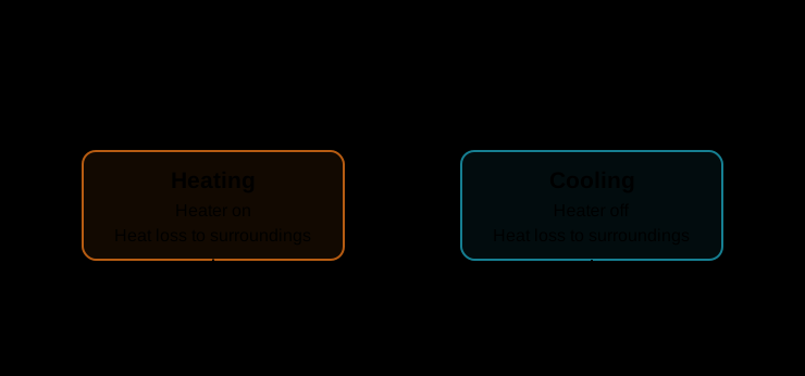
A heater switches on and off around a target temperature. Heat loss to the surroundings continues in both locations. The input moves the switching thresholds; it does not directly change the heating or cooling dynamics.
For temperature \(T\), ambient temperature \(T_a\), heat-loss coefficient \(k\), and heating contribution \(P\),
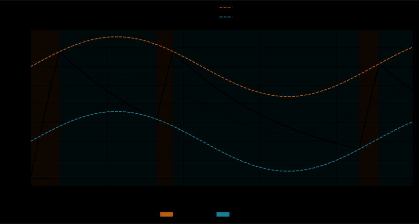
For target temperature \(r(t)\) and hysteresis half-width \(b\), a rising zero crossing of \(T-(r+b)\) switches to cooling; a falling zero crossing of \(T-(r-b)\) switches back to heating. Neither transition resets the temperature.
The illustrated run uses a varying target temperature:
See the thermostat factory for parameter options and the simulation guide for a runnable example.
Bouncing Ball
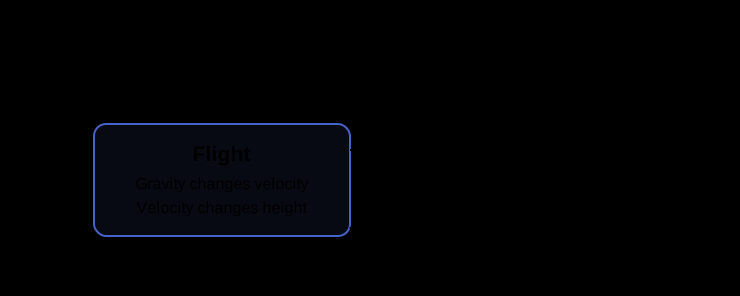
A hybrid system can jump without changing its location. This ball has only one location, flight; impact applies a velocity reset and returns to that same location.
The state is height and vertical velocity, \([h,v]\). Between impacts,
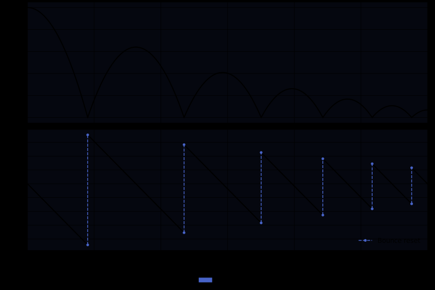
A falling zero crossing of \(h\) detects ground impact. The reset leaves height unchanged and maps velocity to \(v^+=-e v^-\), where \(e\) is the restitution coefficient. There is no resting location in this model.
The illustrated ball is dropped from rest and loses energy at each bounce. Height is interpreted in metres and time in seconds.
See the bouncing_ball factory for gravity, restitution, and initial-state options.
Hybrid Oscillator
An oscillator changes its damping when position crosses the origin. The left and right locations use different damping coefficients but share the same restoring law. Neither position nor velocity is reset at a switch.
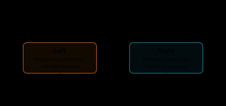
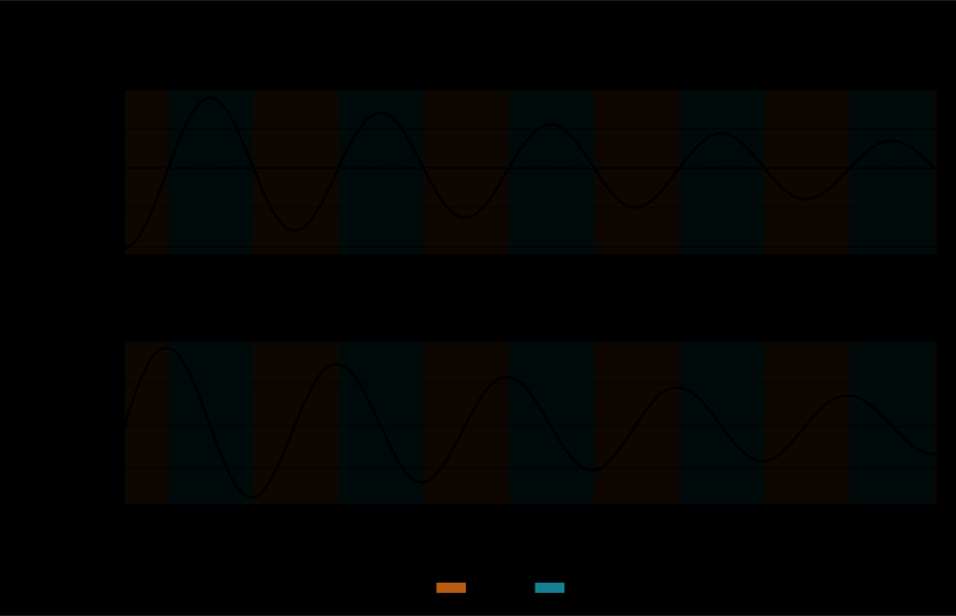
See the hybrid_oscillator factory for parameters.
Switched Linear
This system selects between two linear flows, \(\dot{x}=A_qx\), where \(q\) is the active location. A downward crossing of the first coordinate through a threshold selects off; an upward crossing selects on. These are names for the two dynamics, not an external control input.
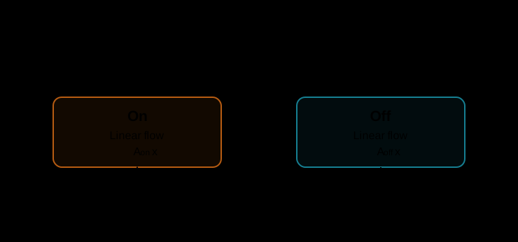
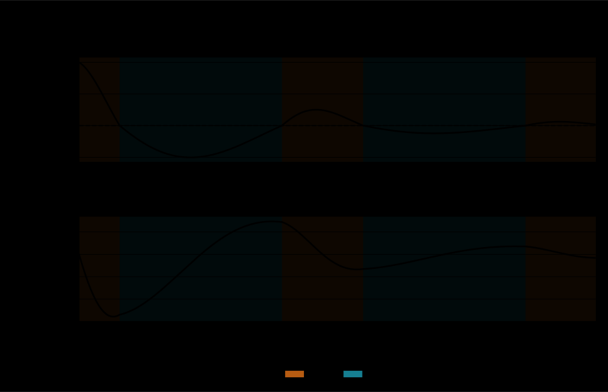
See the switched_linear factory for matrix and threshold options.
Relay Integrator
An integrator alternates between positive and negative constant rates. A rising crossing of the upper bound switches from up to down; a falling crossing of the lower bound switches back. The separated bounds create hysteresis.
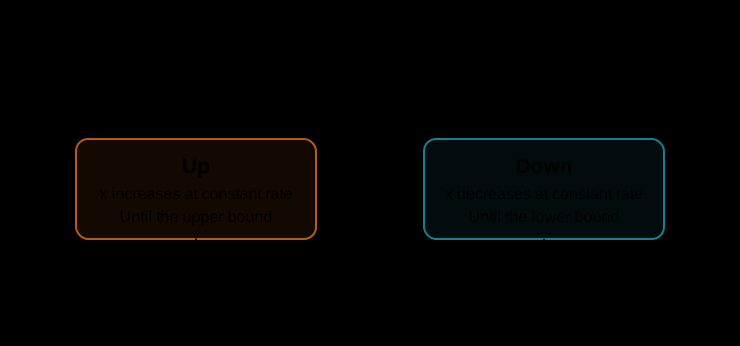
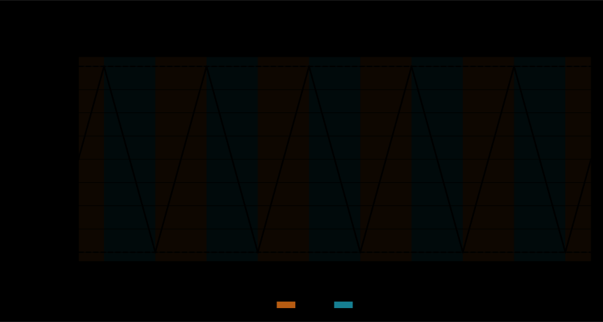
See the relay_integrator factory for slope and bound options.
Time-Varying Event Surface
An input signal moves the switching boundaries around the first state coordinate. The locations apply opposing drift terms and shared damping; the input changes the event surfaces, not the flow laws. The second coordinate decays independently.
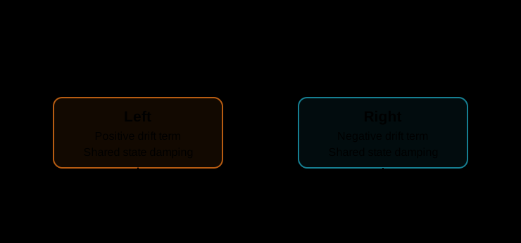
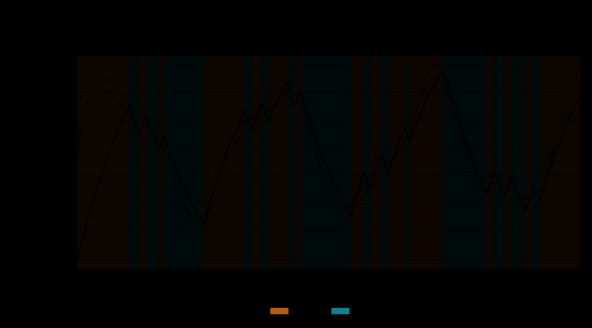
See the time_varying_event_surface factory for its threshold input and parameters.
Time-Forced Switch
Each visit lasts for a fixed dwell time, measured by location residence time. A rising crossing of location_time - dwell_time alternates between fast and slow. The two continuous-state coordinates approach zero more quickly in fast than in slow; neither resets at a transition. The factory's period spans a complete fast-slow cycle.
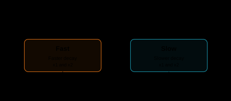
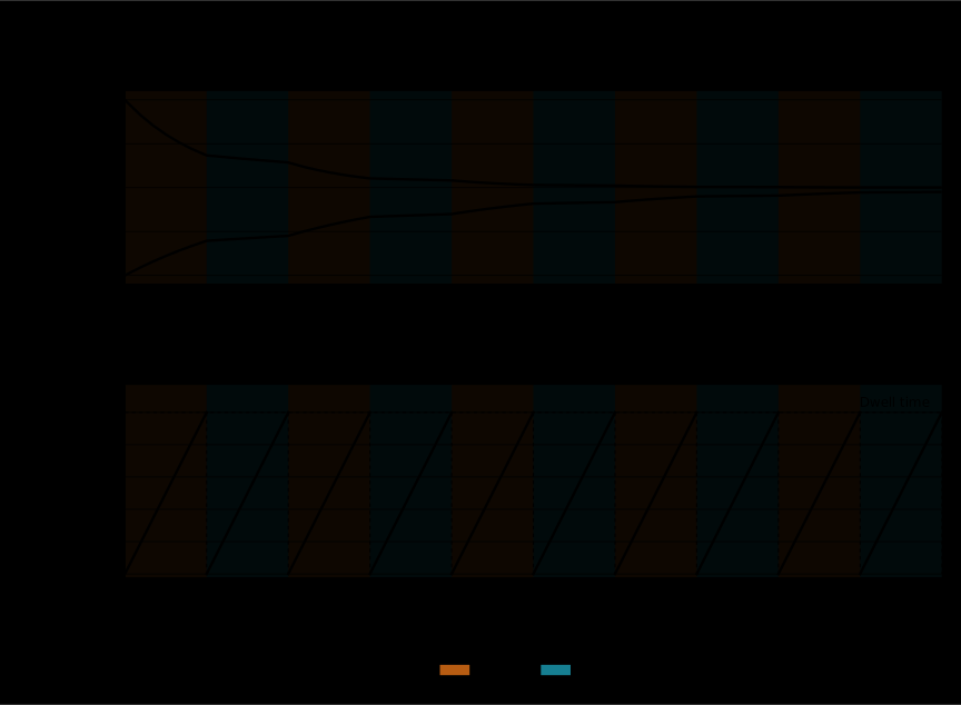
See the time_forced_switch factory for period and initial-state options.
Piecewise Affine
Each location \(q\) defines an affine flow,
with a matrix \(A_q\) and an offset \(b_q\). Crossing a threshold with the first coordinate selects left or right. The threshold is shared by both directions; switching does not reset the state.
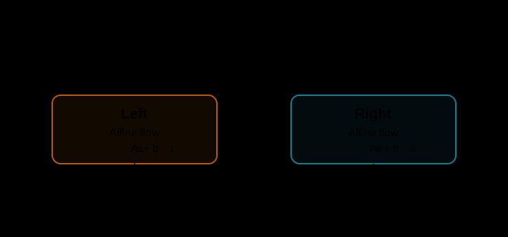
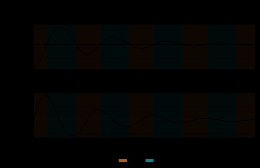
See the piecewise_affine factory for matrices, offsets, and threshold options.
Impact Oscillator
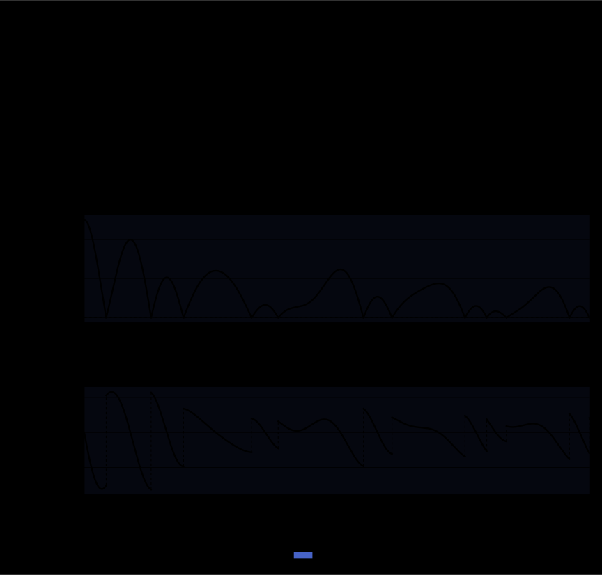
A damped oscillator is driven by a time-varying force and collides with a stop. Position and velocity evolve continuously between impacts. A falling position-zero crossing applies the reset \(v^+=-e v^-\), leaving position unchanged and remaining in the same oscillate location.
See the impact_oscillator factory for the force input and model parameters.
Duffing Oscillator
This idealized unit-mass oscillator represents a mass acted on by a nonlinear spring, a damper, and an external drive. Its state is position and velocity, \([x,v]\), and its input \(u(t)\) is applied force per unit mass. All quantities use normalized units; the model does not prescribe an SI scale.
In location \(q\), the motion follows
The signed linear coefficient \(k\) is shared. Both damping \(d_q\) and cubic stiffness \(c_q\) change between high_damping and low_damping; the location names describe damping, not the entire restoring law. Negative linear stiffness pushes away from the origin at small displacements; positive cubic stiffness pulls back at larger ones.
The locations switch hysteretically on either side of the origin. Moving toward the origin across either inner boundary selects low_damping; moving away across either outer boundary selects high_damping. Between those boundaries, the active location depends on the previous motion. Each switch preserves position and scales velocity by the retention coefficient, reducing speed without reversing its sign. These are switching losses, not collisions with a stop.

The illustrated run applies a cosine force:
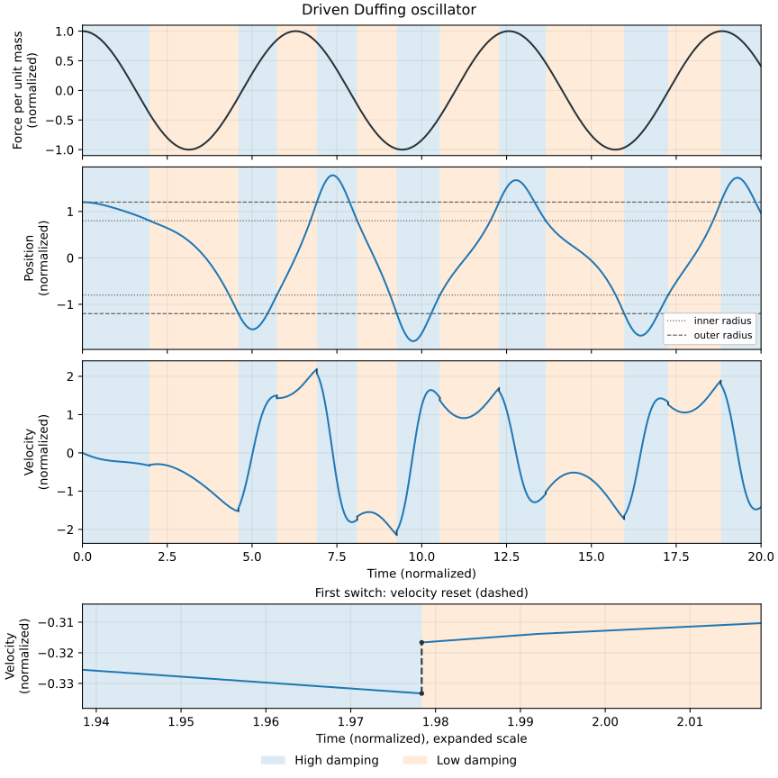
This hybrid variant follows Example 1, Figure 2(a) in the Dainarx paper. Flowcean simulates directed boundary crossings rather than treating the paper's guards as urgent inequalities. See the duffing_oscillator factory for initialization, parameter, and input contracts, and the gallery scenario for forcing and simulation settings.
PID-Controlled Plant
A PID controller drives a second-order plant. Its state contains position, velocity, and the integral of tracking error. The input supplies a reference and its time derivative.
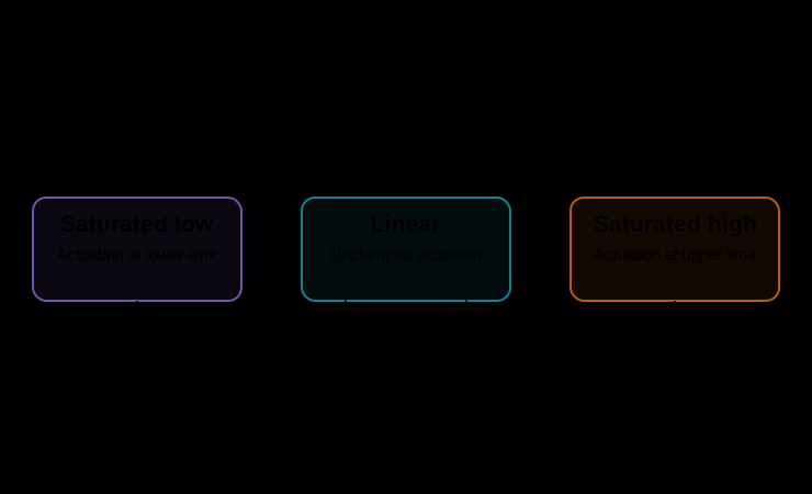
The active location determines whether actuation follows the raw PID command or is clamped at an upper or lower limit. Crossing a limit switches between linear and saturated operation without resetting the state.
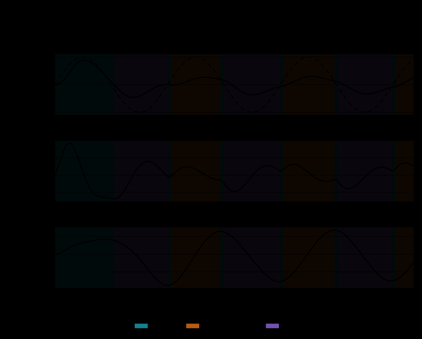
See the pid_controlled_plant factory for gains, actuation limits, and input requirements.
Tank Valves
A pump feeds the first tank while an outlet drains the second. A valve between them opens and closes according to the first tank's level. When open, it permits one-way transfer driven by the level difference.
Closed operation distinguishes a wet second tank from an empty one. When that tank drains to zero, a reset sets its level exactly to zero and the closed_dry location holds it there until the valve opens.
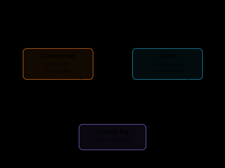
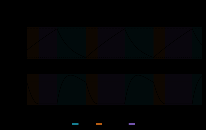
See the tank_valves factory for tank geometry, flow parameters, and switching levels.
Location Cycle
Locations form a cyclic sequence, each applying a different linear flow to the continuous state. When location residence time reaches the dwell time, the system enters the next location at age zero without resetting the state. The factory can vary both the number of locations and the state dimension; the illustrated dimension=3 run has three continuous-state coordinates and no clock coordinate.
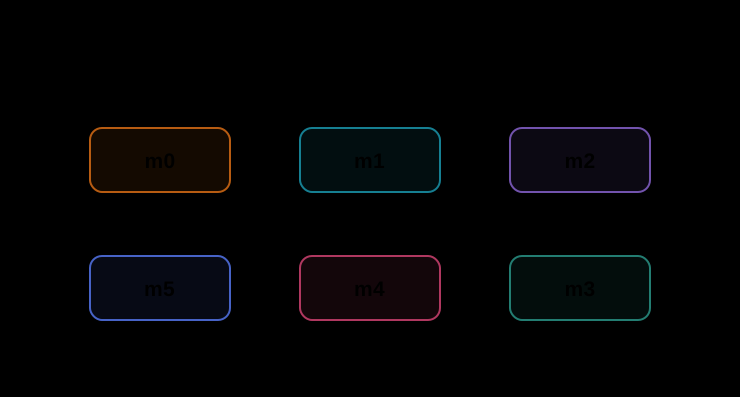
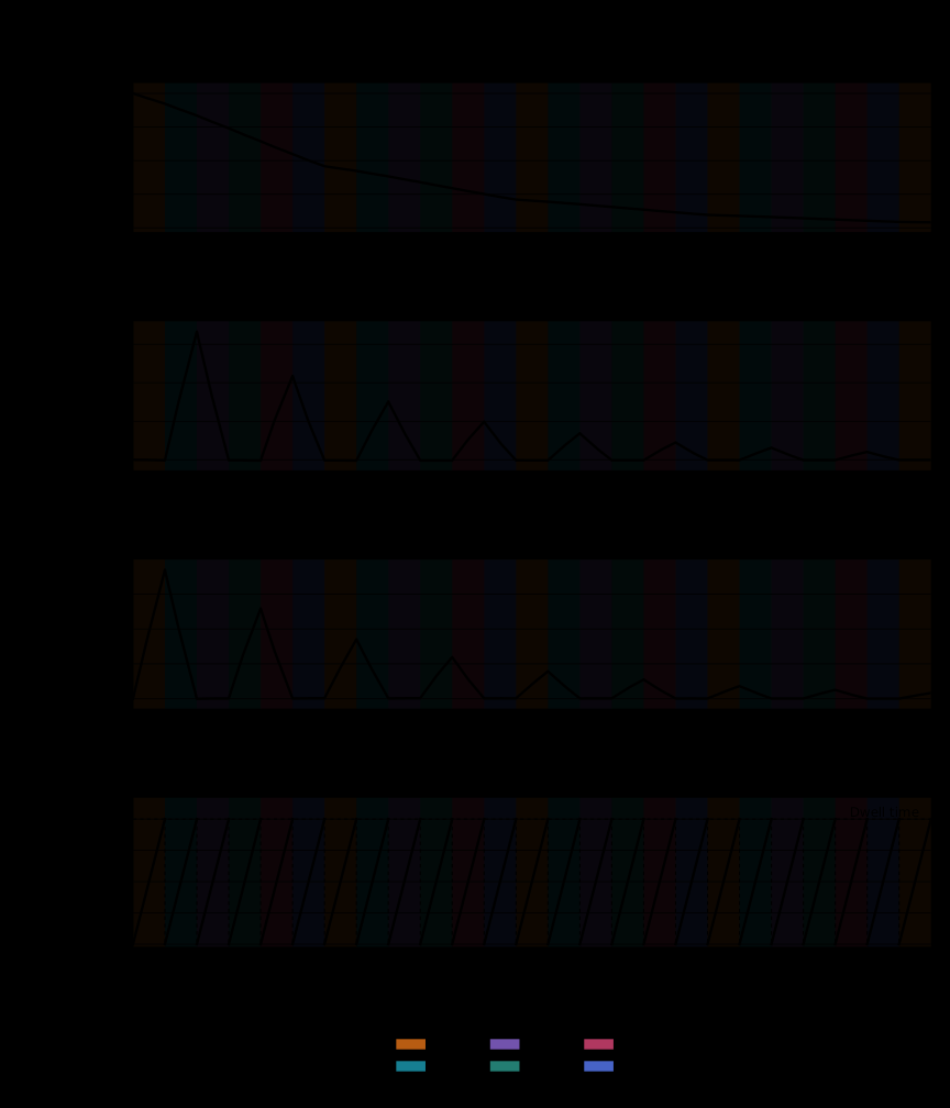
See the location_cycle factory for location count, state dimension, and dwell-time options.
Buck Converter
A buck converter alternates between connecting the supply and letting inductor current freewheel through a diode. Voltage hysteresis determines when the switch opens and closes; there is no fixed-frequency clock.
When the freewheeling current reaches zero, the diode blocks reverse current. The capacitor then supplies the load until output voltage falls to the lower switching threshold.
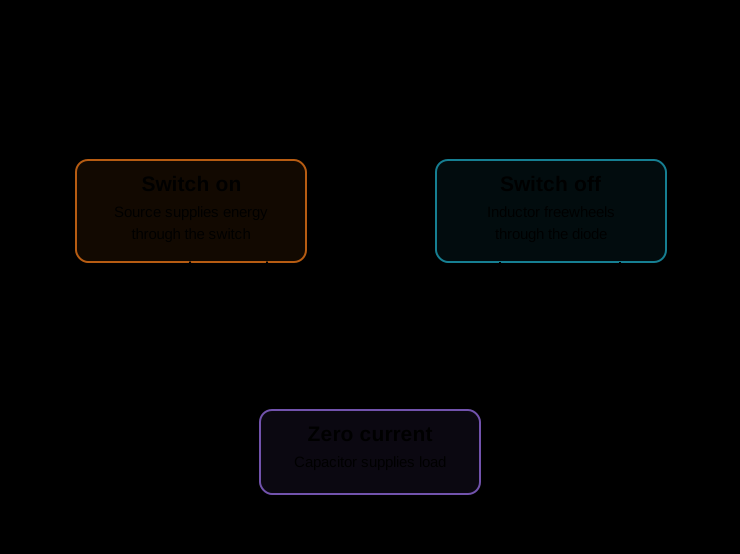
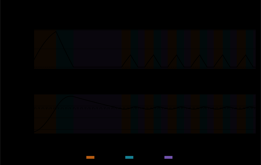
See the buck_converter factory for circuit parameters, conduction laws, and threshold options.
Wind Turbine
This already-running turbine couples rotor motion, tower motion, and blade-pitch control. Its controller switches between generator torque laws without resetting the continuous state.
The state captures rotor speed, tower displacement and velocity, blade pitch and pitch rate, and the pitch controller's integral contribution. The input is wind speed. Generator speed determines the active torque regime; pitch control operates across all regimes.
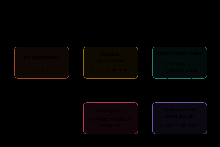
In the illustrated run, wind speed rises and then falls. The plots show how the rotor, pitch controller, and tower respond:
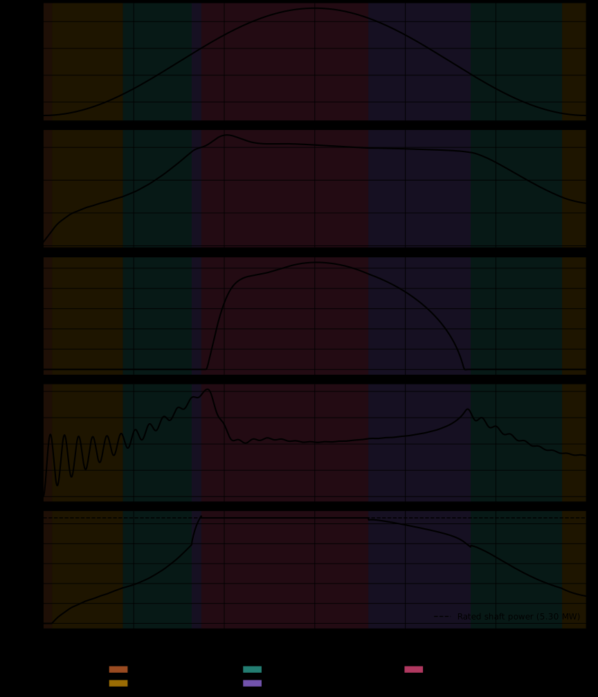
The model assumes quasi-steady, head-on aerodynamics and a running rotor. It does not model startup, shutdown, or emergency braking. Aerodynamic-domain violations stop simulation rather than extrapolating the fitted coefficients. To compute generator-shaft power, pass rotor angular speeds in rad/s, matching location labels, and the turbine's parameters to wind_turbine_power(rotor_speeds, location_labels, parameters=system.parameters). The location selects the torque law even when hysteresis makes speed ambiguous. See the wind-turbine reference for equations, controller parameters, and operating limits.
Run the standalone example to print location changes and save a plot:
Its output is examples/hybrid_systems/outputs/wind_turbine.png.
Delayed Valve Closure
The valve_closure benchmark fills a tank at a constant rate. When the water reaches the closing threshold, the inlet valve closes after the configured delay. Filling continues during the delay, so the final water height exceeds the threshold.
The trajectory records threshold detection in event.detection_time and valve closure in event.time. The delayed-closure scenario appears at the end of the gallery.
Run the Gallery
Run every configured example and save a combined plot to examples/hybrid_systems/outputs/benchmarks.png:
The model configurations and input signals are in scenarios.py.
For a dedicated Duffing plot with an expanded velocity reset, run:
This writes examples/hybrid_systems/outputs/duffing_oscillator-trace.svg. Use --output to select another path or image format. To regenerate its gallery trace from the same scenario:
uv run --directory ./examples/hybrid_systems python duffing_oscillator.py --output ../../docs/assets/hybrid_systems/duffing_oscillator-trace.svg
To work with an installed Flowcean package rather than the repository scripts, start with the simulation example. The identification walkthrough shows how to learn a hybrid model from simulated traces.
Export Automaton Diagrams
To inspect the implemented models, export every example's declared automaton without simulating it:
This writes one DOT file per example under examples/hybrid_systems/outputs/automata/. Add --svg to render SVG files; this requires Graphviz's dot executable on PATH.
The Duffing gallery diagram is the generated outputs/automata/duffing_oscillator.svg; after an SVG export, copy it to docs/assets/hybrid_systems/duffing_oscillator-automaton.svg to update that illustration.
For programmatic export and label options, see build_hybrid_system_dot and render_dot_svg.